In my last post I showed how you can get a bell curve starting with any real number, in only three tiny steps.
This time I want to get a bit more practical, or at least hands-on. You've heard of a bell curve (or normal distribution, Gaussian, etc). Not only that, but you've been put on bell curves at various times, and inspected many other bells to understand aspects of the world. We all know this is a basic measurement and a shape that shows up, well, all over the show.
Why?
I want to explain that simply.
Briefly, a bell curve describes a sum of random influences. Height is normally distributed (in other words on a bell curve) because many little random-ish factors (genes, nutrition, etc) combine to produce your total height—and everyone else's, for that matter, and the same would go for any species. If you're an alien, chances are strong that height for your kind is normally distributed, not to mention many other measurements.
But let's start simple. Let's roll the ol' die.
/https://public-media.si-cdn.com/filer/d1/a1/d1a1820a-25bb-4490-b180-341db209dce2/roman_dice_img_4367.jpeg)
(Wikimedia Commons)
We got 4. But we could have gotten 1, 2, 3, 4, 5, or 6. I'm assuming you thought of a 6-sided die first, and that's what we're using. (By the way, that die is from ancient Rome, so it actually is "ol'.")

(Academo.org)
Here's what things would look like over many rolls: 6 equally likely outcomes. If we kept a tally, it would look lopsided at first, but we wouldn't expect any of the 6 numbers to pull ahead and stay ahead. (See above.) Actually, the longer we kept a tally, the more the race would be neck-and-neck. (That's what the law of large numbers says. See below.)

(Academo.org)

(Xactly.com)
What if we roll 2 dice, though?

(Unknown Source)
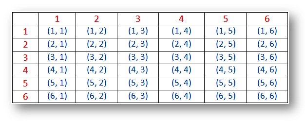
At first, we're going to ignore the green and pink. There are 36 total outcomes (6*6=36) arranged above. As with the single rolls previous, all of these 36 rolls are equally likely. That's important, so I'll say it again: every square (representing a pair of rolled dice) in the chart is equally likely. Here's a chart that makes them look the same.
(Math-Only-Math.com)
(Just a heads-up, between here and the pictures of black dominoes below, we're taking an illustrative detour that you can skip and come back to later. It helps with filling in and seeing the whole picture from end to end.)
Ready? If we go deeper with two dice, the landscape changes. First, notice we could tell the difference between the dice before, as if each had its own size, color, and personality. This was indicated by the dice on the left, which are really just different faces of one die (call it "Left"), and the dice along the top, which are just faces of the other die (call it "Top"). We know which is which. When we roll both dice, the "Left" number is shown on the left between parentheses, like an x-coordinate, and the "Top" number is shown on the right, like a y-coordinate. If we can tell them apart, there are 36 outcomes. But if we can't, only 21 outcomes appear.
Ok. We shall now require our experienced roller of dice to treat all colors as equal. Just to be clear, in this color-equal scenario, rolling 2 and 4 will be the same as rolling 4 and 2. That combination is different from 1 and 5 (which is the same as 5 and 1). Even though all four pairings add up to 6, we'd count two distinct combinations, which I'll call 2&4 and 1&5.
Notice that when both dice come out the same, there's only one way it could have happened. In the chart above, there's (1, 3) and (3, 1), which are the same combination. But there's only (3, 3) once, (4, 4) once, (5, 5) once, etc. So you're twice as likely to get the combination 3&1 as you are to get 3&3.
Let's recap. If we only care about the actual numbers on the dice, meaning we don't care about the colors of the dice, or which die is to the left and which is to the right, etc, then we no longer have outcomes that are all equally likely. This is an artifact of combining two dice which can be mistaken for each other, or at least which are allowed to work exactly the same: there is no priority, rank, order, favorite, etc. One die is as good as another—it doesn't matter which has the 2 and which has the 3. I'm belaboring the point because an interesting transition has happened.
As mentioned earlier, there are 21 of these results that are no longer equally common. The calculation that leads to 21 is technically a combination with replacement (specifically, "6-combinations-of-2 with replacement," the 6 because of 6 sides, the 2 because of 2 dice, and with replacement because both dice are always put back, so they can start out the same from roll to roll).
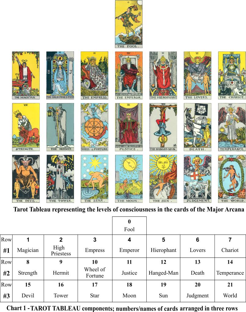
This way of counting does show up materially. It shows up in nature. And it shows up in games, which, after all, are the birthplace of probability and statistical theory (traceable to a letter exchange between Blaise Pascal and a gambler who asked for his help). For example, dominoes began a millennium ago as frozen die rolls for two dice, and they soon evolved into playing cards. The normal 52-card deck has come to reflect 52 weeks in a year. But tarot cards preserve their origins. A deck of tarot cards has 21 trumps, a zero card, and 56 pip/court cards. 6-combinations-of-2 is 21, and 6-combinations-of-3 is 56. So a tarot deck can be seen as a group of cards representing all the rolls of 2 dice, another group representing all the rolls of 3 dice, and then a 0 that's a wild card.
Here are 21 trumps and the 0, for good measure. Bet you never thought of them as dominoes before. (Try to pretend it doesn't talk about "levels of consciousness.")
(Triple 7 Center)
The original Chinese domino sets have 21 types of dominoes for precisely this reason. Meanwhile, traditional European dominoes come in sets of 28 and include 0 as a possible "roll" for each die, so a full set would correspond to all the frozen rolls of a pair of 7-sided dice. True to form, 7-combinations-of-2 is indeed 28. But let's set these aside. The rolls of 0 bring somewhat more confusion than the lone 0 card in tarot. The takeaway is that cards, dominoes, and dice are closely related, and they're all excellent mental tools for thinking about probability and statistics.
In the image below, the upper group of Chinese dominoes is doubled up (two of each kind), while the lower group is made of singletons. We can ignore the decorative colors. There are 32 dominoes in all, but you'll see 21 types. (Specifically, there are 11 different civilian dominoes, and remember that number 11, because it comes up in a second. And there are 10 different military dominoes.) The doubling up doesn't follow the same logic as I talked about above—things get shuffled around a bit—but a glance shows that some pairings (patterns from the civilian suit, for example 1&3) are twice as common/likely as others (patterns from the military suit, for example 2&4).
(LearnPlayWin.net)
Curiously, they even have names. Here are just the 21 Chinese domino types. Again, these embody all the rolls of two dice if you don't care which die is which. Hey, bet you didn't see ancient names like "Copper Hammer Six" on your radar!

(Amazon)
That was a bit of a detour just to reflect on what happens when two dice act like identical twins with the same name: almost counter-intuitively, equally likely faces of a cube give way to unequally likely patterns of pairing. Structure emerges. Possibilities begin to pile up here and not there. Multiple paths lead to the same result. The change is relevant to the creation of a bell curve.
Let's get to the really interesting part. When you add the dice, there will only be 11 possible sums. These are the numbers in the squares in the first chart, which I'll bring back to make things easier.
(Unknown Source)
The sums will go from 2 (ie, 1+1) up to 12 (ie, 6+6), which means there are 11 of them. (If you took the excursion above, remember when I said 11 would come up soon? Not too surprisingly, early on, 11 was the number of cards in a suit. The chain goes: 11 distinct sums with a pair of dice, 11 dominoes in the doubled up civilian suit, 11 cards in the early card suits. It's cultural evolution!) Our transition by the route of adding is important, too: we've gone from 36 outcomes, total, and those are equally likely (called "microstates"), to 11 after adding the faces of the dice, and those sums are not equally likely (called "macrostates" because they can include many microstates). If you look at the grid above, you'll see that 7 occurs more often than 10 as a sum. There are more ways to get to it. So if you ever have a chance to bet on the sum of two dice, bet on 7 and you'll win more often than anyone choosing other bets. As it so happens, 7 is the mean, median, and mode, and it's six times more likely than 2 or 12.
To use the terminology just introduced, 7 and 10 are two different macrostates. The macrostate of 10 covers only 3 microstates, but the macrostate of 7 covers 6 microstates. I like to avoid jargon, but these three levels of thinking about a pair of dice (36 equal microstates/permutations-with-replacement, 21 unequal macrostates/combinations-with-replacement, and 11 unequal macrostates/sums) can be confusing to think about. It really helps to have some words. You can pick whichever you like.

(Xactly.com)
Here is what the outcomes would look like over many rolls. Above is an experiment and below is the idealized, long-term version. Macrostates line the horizonal axis. Each black-and-white pair below is a microstate. (Also, notice the similarity between this way of showing a pair of dice and a domino. Normal dominoes are macrostates of dice, but these ones are microstates, because all 36 permutations are included, and no symmetry is removed.)

(Unknown Source)
Long story short, the picture is no longer flat. It is not a uniform distribution anymore. Taking two die rolls and adding them does something a bit different from just rolling a die with 11 sides, or 21 sides. In fact, we've done something interesting that could look scary, something that involves calculus, but we don't need that right now. By rolling dice and plotting, we've done it. This is called the convolution of two random variables.
Let's convolve again. With one more die, we are convolving three dice together. What does that look like?
(American Scientist)
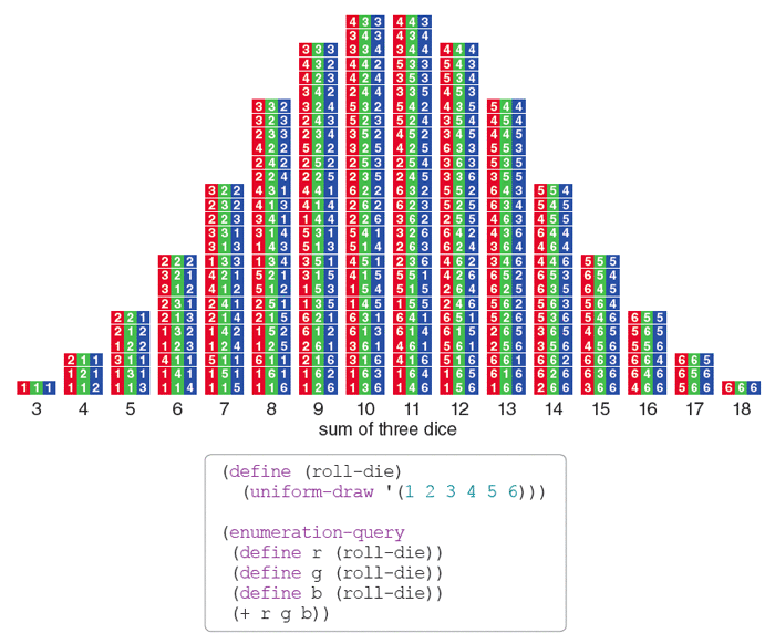
Note that the sums of 3 to 18 correspond to sums of 2 to 12 with two dice. (Meanwhile, and not shown, there are 56 clearly different combinations for three dice, corresponding to the 21 combinations for two dice discussed earlier; relatedly, there are 56 suit cards in a tarot deck, and 21 trump cards, not including the 0 card.) The chart above uses three colors, one for each die, to show how the triples of dice are ordered into all 6*6*6 = 216 permutations and sorted into sums—3 through 18.
Though the above (that code is Lisp by the way, but we're ignoring it) is not exactly a normal distribution as it's discrete and jagged, it already approximates one. The more dice you throw, the more the histogram will approximate a perfectly smooth bell curve.
(Wolfram MathWorld)
A bell curve is the result of convolving ("adding up") random influences.
The especially interesting thing about bell curves is that even if your dice were weighted for cheating, you'd still get a bell curve. Maybe it makes sense that many fair dice would produce that nice smooth shape, given enough dice. But unfair dice would, also. We'll say more about those dice in a second, but let's divert to the real world first.
When you're adding up the influence of genes and nutrients and so on to get a person's final height, it doesn't really matter how common the genes are compared to each other, for example. Some variants could be rare, others common. When you add up their influences, you'll still get a bell curve.
And how often do random factors add up to something? Very! That's why the shape is so common!

(Xactly.com)
It turns out that as long as the dice (random variables/factors) behave something like physical dice, then convolving enough of them will produce a bell curve. What dice would not be allowed to do is lack an average value and a standard deviation. If the die had infinitely many sides, for example, this wouldn't work.
As a consequence, when you see a bell curve, you can conclude that the main contributing factors, even if they're really quite random, all have well-defined averages and standard deviations. The random variables may or may not themselves look like bell curves when analyzed individually. They could be uniformly distributed (flat) like a single die. They could be noisily scattered within a band of possible values. Or the weighting could be anything else that has a finite, consistent average and standard deviation. Bell curves show up everywhere because when you add up randomness, it's very difficult to avoid them.